The secrets from within the USA Ultimate ranking algorithm.
January 21, 2015 by Scott Dunham in Analysis with 20 comments
There are two complaints I have seen repeatedly in Ultiworld comments and elsewhere:
- “My team doesn’t have a chance to earn a bid because we can’t get into the top tournaments”;
- “Team X is ranked higher than they should be because they only/mostly played weaker teams.”
Of course, these two complaints seem contradictory, which motivated me to examine the data to see whether either of them is justified. In the course of answering that question, the analysis also provides some insight into whether and how the algorithm should be improved to make it fairer to all.
Last year, Scott Shriner published two articles on Ultiworld analyzing how a team might maximize its ranking and trying to identify which tournaments a team should attend in order to earn a strength bid. The problem with the analysis in both of these articles is that it does not account for how these two components of ranking are coupled. Clearly, teams can be expected to win more often and by larger margins against weaker teams. The question is whether the increase in expected Rating Differential from the USAU algorithm is sufficient to offset the lower opponent Team Rating.
As an example, if Team 1 is ranked 1800 and Team 2 is ranked 1600, then Team 1 is likely to win. However, if Team 1 only wins on double game point, then the Game Differential would be just 125, so the Game Rating for Team 1 would be 1600 + 125 = 1725. This is lower than Team 1’s current rating and so their rating would drop. For Team 2, the Game Rating would be 1800 – 125 = 1675, so this game would boost Team 2’s rating. I call the amount by which a Game Rating differs from a participating team’s rating the Net Game Rating (-75 for Team 1 and +75 for Team 2 in this example).
If we average all the Net Game Ratings for games between teams about 200 points apart in rating, we can see whether in such match-ups it is better to be the stronger or weaker team (ideally it wouldn’t matter). I calculated these averages for the full range differences between team ratings (Net Team ratings).
For those of you who want a few more details, here is what I did in order to explicitly account for the coupling between results and strength of schedule:
1. I started with the full set of 2014 regular season college men’s and women’s game results as provided by USAU1 , 2
2. For each game, I calculated a Net Team Rating (Team 2 Rating – Team 1 Rating) and a Net Game Rating (Game Rating – Team 1 Rating) 3 , 4
This analysis allows us to see how opponent strength impacted distribution of game rating: which types of opponents (for example, “much stronger” or “slightly weaker” or “essentially even” opponents) were likely, on average, to raise or lower ranking. In order to more clearly see the trends, games were ordered by Net Team Rating and then smoothing5 was used to calculate moving averages for both Net Team Rating and Net Game Rating6, 7. The results are shown in figures below.
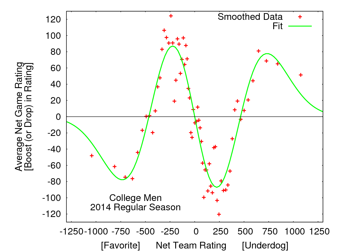
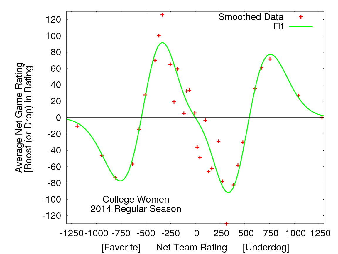
Figure 1: Moving averages of Net Game Rating versus Net Team Rating for Men (above) and Women (below) during 2014 College Regular season. Each point represents an average over 100 games with similar Net Team Ratings.
Looking at these plots, some broad trends emerge.
1. It was advantageous to play teams that were moderately weaker (up to about 500 points lower) and therefore a disadvantage to play teams that were moderately stronger.
2. It was disadvantageous to play teams that were much weaker (more than about 500 lower), and therefore an advantage to play teams that were much stronger.
Returning to the example above, these plots say that during the 2014 college regular season a Men’s/Women’s team ranked 200 points higher than its opponent received on average a Net Game Rating about 80/60 points higher than their season average for that game. Conversely, a team ranked 200 points lower than its opponent had an average Net Game Rating about 80/60 points lower than its rating.
Taking another example, playing a team ranked about 1000 points lower resulted in an average Net Game Rating about 50 points below a team’s final regular season rating. However, it is important to note that these advantages/disadvantages are far from a sure thing, as the variances in the data were very large.8 For example, Men’s teams with ratings about 200 points higher than their opponents have an average Net Game Rating of about +80, but 27% of the time, those teams lost ratings points in these matchups.
For teams ranked moderately lower, the Game Differential is (on average) more than enough to compensate for the rating difference. However, since the maximum Rating Differential in the current algorithm is 600 points, playing teams rated more than 600 points lower can only lower a team’s rating, and there are minimal gains (along with the risk of significant losses) possible when playing teams ranked close to that threshold. Note that the results analyzed here are limited to a single season since the algorithm was changed in 2014.9
The advantages/disadvantages shown in the figures are relatively modest (especially in relation to the standard deviations), suggesting that the current algorithm gives quite reasonable results. In fact, when the corrections given by the fit to the data (green lines in the figures) were applied to 2014 team rankings, the allocation of strength bids was unchanged. However, the analysis does suggest some directions in which the algorithm might be improved.
First, it seems there should be the possibility of a small gain for the higher ranked team when beating a much lower ranked team by a sufficient margin. This would balance out the otherwise one-sided cost of not winning by more than 2 to 1. It would also be helpful to reduce the weighting of these games.
Second, it should be possible to mostly eliminate the biases associated with Net Team Rating for moderate rating differences by optimizing the Game Differential point values used in the algorithm based on historical (or even current season) data. For example, in current system winning by two in a game to 13 is worth almost twice as much (+229) as winning by one (+125).
In a capped game to 10 or less, winning by two is actually worth more than twice as much as winning by one. If this difference (and also differential for winning by three) was reduced, then the advantages of playing a moderately lower ranked team might be reduced.
Returning to the questions raised at the beginning of the article, this analysis gives pretty clear answers.
First, teams are not disadvantaged (at least in terms of earning strength bids) by not getting access to top tournaments. In fact, missing these tournaments likely increases the chance of a team earning a strength bid for their region. At top tournaments, a team near the bid threshold will mostly be playing teams ranked above them, and as seen in the figures, these games have a negative Average Net Game Rating; on average, these games drop a team’s rating10.
There does, however, seem to be a modest advantage in playing a relatively (but not too) weak schedule. The prescription for choosing tournaments to maximize ranking is pretty simple and seems very sensible: teams should go to tournaments at which they can do well, but still get a reasonable challenge.
Thanks to Ty Krajec and Steve Wang. ↩
I deleted all games which involved a team which didn’t qualify for ranking (and therefore had no Team Rating) or for which there was no score (e.g., W-L or W-F). ↩
Remember that the Game Rating is the sum of Team 2 Rating and the Rating Differential calculated from the game score using the USAU Ranking Algorithm (http://play.usaultimate.org/teams/events/rankings/). ↩
One more methodology note: I set the Net Game Rating to 0 for all games which get near-zero weight due to Net Team Rating greater than 600 and win by more than 2 to 1. ↩
Net Team Ratings and Net Game Ratings for 100 games were averaged to generate each data point shown in plots with a data point taken each 50 games (e.g. points are plotted for average of games 1-100, 51-150, etc.). ↩
I also fit the data to a smooth function chosen to match the observed behavior: Cx(x2-b2)(x2+d2)exp(-ax2), with C, b, d, and a fit to the data. ↩
All games are listed twice with Teams 1 and 2 reversed so data is presented from the perspective of both teams.[1] Thus the data is “odd” by construction (if –x,-y is in the data set, then so is x,y). The window-smoothed data shown in plots is not perfectly symmetric due to offsets in the window ranges used. ↩
The standard deviation in the Net Game Rating peaked at about 400 points for equally matched teams, dropping to about 150 points for mismatches. Since the standard deviations are much larger than the averages, the favored team loses rating points much of the time. ↩
However, we conducted a similar analysis of partial data (only teams near the bid threshold) for the 2013 season and the results were very similar. ↩
Of course, to be clear, the reason these games on average drop a team’s rating is because, on average, the team is likely to lose these games ↩